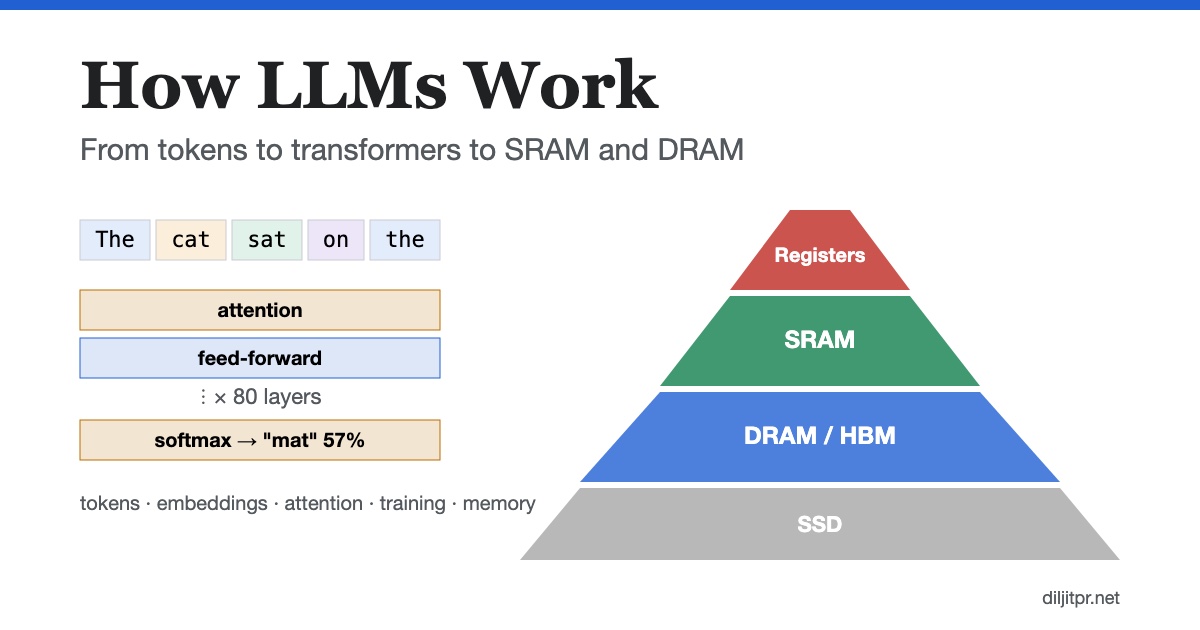
A large language model (LLM) is a program that predicts the next piece of text. It splits your words into tokens, turns each token into a list of numbers, passes those numbers through dozens of layers that let every token look at the ones before it, and outputs a probability for every possible next token. It picks one, adds it to the text, and repeats. ChatGPT, Claude and every other chatbot work this way.

That one loop explains everything else, including why these models need so much memory, and why the difference between SRAM and DRAM decides how fast they talk. This post starts from zero and goes deep. It follows one sentence, "The cat sat on the", all the way through a model, with real numbers you can check by hand. No maths beyond multiplying and adding is needed.

Part 1 · The big picture

What does an LLM actually do?

An LLM does one thing: given some text, it predicts what comes next. It is autocomplete, made very large and very good. Ask it a question and it doesn't look up an answer. It predicts the first token of a likely reply, then the next, then the next, until it predicts a "stop" token.

This is called next-token prediction, and producing text one token at a time, feeding each output back in, is called autoregressive generation. It sounds too simple to produce essays and code. The trick is that predicting the next word well, across trillions of words of text, forces the model to learn grammar, facts, and the patterns of reasoning that text contains.

What is a "model", and what are parameters?

A model is a mathematical function: numbers go in, numbers come out. What it computes is set by adjustable numbers inside it called parameters or weights. Here is the smallest possible model, with two parameters:

prediction = w × input + b

// w and b are the parameters. Training finds the values that make predictions right.
// e.g. predicting a house price from its size: w = price per square metre, b = base price.

An LLM is the same idea with billions of parameters instead of two, arranged into big grids of numbers called matrices. When you read "Llama 3 70B", the 70B means 70 billion parameters. The parameters are the model: the program that runs them is short, and the file you download is almost entirely these numbers.

Part 2 · From text to numbers

What is a token in AI?

A token is the unit of text an LLM reads and writes: a whole common word, a piece of a rarer word, a space plus a word, or a punctuation mark. Models work on tokens rather than letters or words because tokens strike a balance. Letters would make sequences very long; whole words would need a vocabulary of millions and still miss new words.

A tokenizer splits text into tokens using a vocabulary learned from data, usually with a method called byte-pair encoding (BPE), which starts from single characters and repeatedly merges the most common pairs. The result might split a sentence like this:

(The dot marks a leading space, which is part of the token.) Common words are one token; "unbelievably" is three. Each token has an ID number in the vocabulary, and the model only ever sees those IDs. Some reference points:

• According to OpenAI's guidance, one token is about 4 characters or three quarters of a word of English text, so 1,000 tokens is roughly 750 words.
• Vocabularies hold roughly 100,000 to 200,000 tokens. Llama 3 uses 128,000; OpenAI's GPT-4o tokenizer uses about 200,000.
• Other languages and code often need more tokens per word, which is why the same message can cost more in Hindi than in English.

What are word embeddings?

A token ID like 8415 is just a label; the number itself means nothing. So the first thing a model does is look each ID up in a table, the embedding table, and swap it for a list of numbers called an embedding or vector. In a large model each vector holds thousands of numbers: 4,096 in Llama 3 8B, 8,192 in Llama 3 70B.

Those numbers are parameters, learned during training. Training pushes tokens used in similar ways toward similar vectors, so meaning becomes geometry: "cat" ends up near "dog", far from "spreadsheet". Directions can carry meaning too, which is the famous "king − man + woman ≈ queen" result from word2vec.

One more ingredient: word order. "Dog bites man" and "man bites dog" contain the same tokens. Models add position information so each vector also encodes where its token sits. Most current models use RoPE (rotary position embedding), which rotates parts of each vector by an angle that depends on position.

Embeddings are also what powers search by meaning in retrieval-augmented generation (RAG).

Part 3 · Inside the transformer

What is the transformer architecture?

The transformer is the design almost every LLM uses, introduced by Google researchers in the 2017 paper "Attention Is All You Need". It is a stack of identical layers (32 in Llama 3 8B, 80 in Llama 3 70B). Each token's vector flows up through the stack, and each layer adds something to it.

A useful picture is a conveyor belt called the residual stream. Each token has its own belt carrying its vector. Each layer reads the belt, computes an update, and adds it back, so information accumulates instead of being overwritten. Every layer has two stages:

1. Self-attention: tokens exchange information with earlier tokens.
2. Feed-forward network: each token is processed on its own, using knowledge stored in the weights.

How does self-attention work?

Self-attention is how a token gathers information from the tokens before it. To predict what follows "The cat sat on the", the model needs the last token to know a cat was sitting. Attention does that in three steps, using three vectors that each token computes from its own embedding with learned weight matrices:

• Query (Q): what this token is looking for.
• Key (K): what this token offers, used for matching.
• Value (V): the information this token hands over if it is chosen.

Think of a library: your query is the question you bring, each book's key is its catalogue entry, and its value is the content. You read most from the books whose catalogue entries best match your question.

A worked example with real numbers

Take three tokens, "The cat sat", and compute attention for "sat". Real vectors have thousands of numbers; here they have two so you can follow the arithmetic. Suppose the weights produce:

Token	Key (K)	Value (V)
The	[0.2, 0.1]	[0, 1]
cat	[1.0, 1.5]	[3, 0]
sat	[0.5, 0.5]	[1, 1]

and the query for "sat" is [1, 2].

Step 1. Score each token with a dot product (multiply matching positions, add them up), then divide by √2, the square root of the vector length, to keep numbers in a sensible range:

The: (1×0.2 + 2×0.1) = 0.4  ÷ 1.414 = 0.28
cat: (1×1.0 + 2×1.5) = 4.0  ÷ 1.414 = 2.83
sat: (1×0.5 + 2×0.5) = 1.5  ÷ 1.414 = 1.06

Step 2. Turn scores into weights that add up to 1 with softmax (explained in detail below): raise e ≈ 2.718 to the power of each score, then divide each by the total.

e^0.28 = 1.33   e^2.83 = 16.9   e^1.06 = 2.90     total = 21.1
weights:  The 6%   cat 80%   sat 14%

Step 3. Blend the values using those weights:

0.06 × [0, 1] + 0.80 × [3, 0] + 0.14 × [1, 1] = [2.54, 0.20]

The output is mostly "cat"'s value. "Sat" has pulled in information about who is sitting. That output is added to the residual stream for "sat", and the next layer works with the richer vector.

Two more facts complete the picture. Multi-head attention runs many small attention computations side by side, so one head can track grammar while another tracks who "it" refers to. And because a token's key and value never change once computed, generation stores them instead of recomputing them; that store is the KV cache, which I cover in depth in KV cache explained with a 3-trillion-parameter model.

What does the feed-forward network do?

After attention, each token's vector goes through a feed-forward network (FFN) on its own. It multiplies the vector by a weight matrix that expands it, typically to about 4 times its width, applies a simple non-linear function that zeroes or shrinks some of the numbers, then multiplies by a second matrix that shrinks it back. Without that non-linear step, stacking layers would collapse into one big multiplication and the model could only learn straight-line relationships.

Many frontier models replace the single FFN with a mixture of experts (MoE): dozens or hundreds of smaller FFNs plus a small router that sends each token to a few of them. The model can hold far more parameters than it uses for any one token. DeepSeek-V3, for example, has 671 billion parameters but activates about 37 billion per token.

Between these blocks sit small normalisation steps (RMSNorm in most current models) that rescale each vector to a steady size so numbers neither blow up nor vanish as they pass through dozens of layers.

Part 4 · Getting an answer out

What is softmax?

After the last layer, the final token's vector is multiplied by one more matrix, the output head or unembedding, which produces one score per vocabulary token. These raw scores are called logits. They can be any number, negative or positive. Softmax is the function that turns them into probabilities: it makes every value positive with e^x, then divides by the total so they add up to 1. It is the same function attention used in step 2.

Here are made-up but realistic logits for the token after "The cat sat on the":

token     logit   e^logit    probability
mat        4.0     54.6      54.6 ÷ 96.1 = 56.8%
floor      3.2     24.5                    25.5%
sofa       2.5     12.2                    12.7%
roof       1.5      4.5                     4.7%
banana    -1.0      0.37                    0.4%
                   ─────
          total    96.1

Because of the exponential, a gap of 0.8 in logits ("mat" vs "floor") becomes more than a 2× gap in probability. Softmax rewards the leader.

What does temperature do in an LLM?

Temperature is a number the logits are divided by before softmax. Below 1, it sharpens the distribution so the top token dominates; above 1, it flattens it so unlikely tokens get a real chance. Then a token is sampled: picked at random in proportion to its probability. Move the slider:

Temperature	mat	floor	sofa	roof	banana	Feels like
0.5	79.5%	16.0%	4.0%	0.5%	<0.1%	focused, repeatable
1.0	56.8%	25.5%	12.7%	4.7%	0.4%	the model's own odds
2.0	39.8%	26.7%	18.8%	11.4%	3.3%	loose, sometimes odd

Temperature 0 means always taking the top token (greedy decoding). Two other common settings trim the tail before sampling: top-k keeps only the k most likely tokens, and top-p keeps the smallest set whose probabilities add up to p (say 90%). Low temperature suits code and data extraction; higher suits brainstorming.

This is also why the same prompt can give different answers: the model's probabilities are the same each time, but the sampling is random.

Part 5 · How it learned

How are LLMs trained?

A new model starts with random parameters and predicts garbage. Training fixes that with a simple loop, repeated billions of times:

1. Take real text from the training data, for example "The cat sat on the mat".
2. Predict each next token from the ones before it (the forward pass).
3. Measure the error, called the loss.
4. Work out how to nudge every parameter to reduce that error (backpropagation).
5. Nudge them a tiny step in that direction (gradient descent).

The loss: how wrong was the prediction?

The standard loss for language models is cross-entropy: the negative logarithm of the probability the model gave to the token that actually came next.

probability given to the correct token "mat"    loss = −ln(p)
90%                                               0.11   almost right
60%                                               0.51
25%                                               1.39
5%                                                3.00
0.1%                                              6.91   badly wrong

Confident and right costs almost nothing; confident and wrong is punished hard. Averaged over trillions of tokens, lowering this one number is the entire training objective.

What is gradient descent?

Picture the loss as a landscape: every possible setting of the parameters is a point, and the height is the loss. Training wants the lowest valley. The gradient is the slope under your feet: for each parameter, which direction increases the loss and how steeply. Gradient descent takes a small step the opposite way, downhill, then measures the slope again.

What is backpropagation?

Gradient descent needs the slope for every one of billions of parameters. Backpropagation computes all of them in one backward sweep. It starts at the loss and walks back through the layers, using the chain rule from calculus to pass blame along: if the output was too low, which numbers in the last layer caused that, and which numbers in the layer before caused those. One backward pass costs about twice as much as the forward pass, and it needs every layer's intermediate results saved from the forward pass, which is why training uses far more memory than running a model.

The stages of training

Stage	Data	What it adds
Pre-training	Trillions of tokens of web text, books, code. Meta trained Llama 3 on over 15 trillion tokens.	Language, facts, reasoning patterns. The result completes text but doesn't follow instructions well.
Supervised fine-tuning	Thousands to millions of example conversations written or checked by people	The assistant format: answer the question that was asked.
Preference tuning (RLHF, DPO)	Pairs of answers ranked by people or by other models	Helpfulness, tone, refusing harmful requests.
Reinforcement learning on tasks	Maths, code and agent tasks with checkable answers	Longer step-by-step reasoning, the basis of "thinking" models.

Training ends and the parameters freeze. Everything after that, every chat you have, is inference: running the frozen model forward. The model doesn't learn from your conversation unless its makers later train a new version.

Part 6 · The hardware

Why is it all matrix multiplication?

Strip away the names and almost every step above is the same operation: multiply a vector, or a stack of vectors, by a big matrix of parameters. Making Q, K and V, the FFN's expand and shrink, the output head: all matrix multiplications. A useful rule of thumb follows from this:

work per token ≈ 2 × number of parameters used   (one multiply + one add each)

70B-parameter model → about 140 billion operations per token

Chips that do huge numbers of multiply-adds in parallel, GPUs and AI accelerators, are therefore the natural hardware. I explain how a GPU does that, with Rust examples, in CPU, GPU and CUDA fundamentals for engineers. But arithmetic is only half the story. Every one of those parameters has to be fetched from memory first.

What is the memory hierarchy?

Computers can't have memory that is fast, large and cheap all at once. Instead they stack several kinds in a memory hierarchy: tiny and very fast at the top, near the compute; huge and slow at the bottom. Data the processor needs right now is copied up the levels.

Level	Typical size	Access time	Built from
Registers	Hundreds of bytes per core	Under 1 ns	Flip-flops in the core
L1 / L2 / L3 cache	Tens of KB to tens of MB	About 1 ns to 40 ns	SRAM
Main memory / GPU memory	16 GB to 192 GB	About 60 to 100 ns	DRAM (DDR, GDDR, or HBM)
SSD	Terabytes	About 100 µs	NAND flash

A kitchen analogy: registers are the ingredients in your hand, SRAM cache is the counter, DRAM is the fridge across the room, and the SSD is the supermarket. Cooking speed depends on how often you walk to the fridge.

SRAM vs DRAM: what's the difference?

SRAM (static random-access memory) stores each bit in a small circuit of about six transistors that hold their state as long as power is on. DRAM (dynamic random-access memory) stores each bit as electric charge in one tiny capacitor, guarded by one transistor. That single design difference explains everything about how each is used.

	SRAM	DRAM
One bit is stored in	About 6 transistors (a latch)	1 transistor + 1 capacitor
Needs refreshing?	No, holds while powered	Yes, about every 64 ms, because the charge leaks
Speed	Fastest; a few cycles	Slower; tens of nanoseconds
Density and cost per bit	Low density, expensive	High density, cheap
Where it sits	On the processor chip itself	Separate chips beside the processor
Used for	CPU and GPU caches, register files, scratchpads	Main memory (DDR), graphics memory (GDDR), HBM
Typical amount	Megabytes per chip (an H100 has 50 MB of L2 cache)	Gigabytes (an H100 has 80 GB of HBM)

Both are volatile: they lose everything when power is cut. That is why model weights are stored on an SSD and loaded into DRAM when the model starts.

What is HBM (high-bandwidth memory)?

HBM is DRAM built for bandwidth. Several DRAM chips are stacked on top of each other (8 to 12 layers in current parts), connected vertically by thousands of tiny wires through the silicon called through-silicon vias, and placed right beside the GPU on a shared base called an interposer. Each stack talks to the GPU over a 1,024-bit-wide connection, compared with 64 bits for a normal DDR memory stick.

The result: an NVIDIA H100 reads its 80 GB of HBM at about 3.35 TB/s, and a B200 reads its HBM at about 8 TB/s. A desktop PC's DDR5 memory manages around 60 to 100 GB/s. HBM is expensive and hard to make, which is why its supply is one of the main limits on how many AI chips get built.

Why do LLMs wait on memory instead of compute?

Now combine the last few sections. When a model generates a token, it must read every parameter it uses from memory, and it does only about 2 operations with each one. Here is a 70B-parameter model in 16-bit numbers (140 GB) on one H100, assuming for simplicity that the whole model fit on it:

memory time  = 140 GB ÷ 3.35 TB/s          ≈ 42 ms
compute time = 140 GFLOP ÷ ~989 TFLOP/s     ≈ 0.14 ms   (H100 dense 16-bit peak)

the arithmetic units sit idle about 99% of the time

Generating text is memory-bandwidth-bound: speed is set by how fast weights arrive, not by how fast they're multiplied. That gives the most useful formula in LLM serving:

tokens per second (one user) ≲ memory bandwidth ÷ bytes of weights read per token

Every major speed trick attacks one side of that fraction:

• Quantization stores weights in fewer bits (8 or 4 instead of 16), so fewer bytes are read per token.
• Mixture of experts reads only the experts a token uses, not every parameter.
• Batching reads the weights once and uses them for many users' tokens at the same time.
• More SRAM: chips like Cerebras's wafer-scale engine keep weights in on-chip SRAM, which is far faster than HBM, by spreading the model across many chips. I worked through how that serves a 3-trillion-parameter model in the KV cache post.

Part 7 · Serving a model

Prefill, decode, KV cache and batching

Answering a request happens in two phases. Prefill processes your whole prompt at once: all prompt tokens go through each layer together, each weight is reused for thousands of tokens, so it is limited by compute. That is the pause before the first word appears. Decode then generates one token at a time, memory-bound as above. That is the speed at which words stream out.

During decode, the KV cache keeps the keys and values of all earlier tokens so they aren't recomputed. It grows with every token and every user, and on long conversations it can take more memory than the weights. Servers use continuous batching to mix many users into each step, and paged attention to store each user's cache in fixed-size blocks so memory isn't wasted.

When a model is too big for one chip, it is split. Tensor parallelism slices each layer across several GPUs; pipeline parallelism puts different layers on different machines and passes each token's vector along. I tried pipeline parallelism across ordinary machines in running a 397B model on 20 GPUs, and measured the CPU-versus-GPU gap on a real model in running half a language model on a CPU and a GPU.

Putting it together: one token's full journey

Here is everything above, in order, for the moment a chatbot writes "mat" after "The cat sat on the":

1. The text is split into tokens and each becomes an ID: The · cat · sat · on · the.
2. The prompt's tokens go through every layer at once (prefill), and each layer saves their keys and values in the KV cache.
3. For the last token, each layer's weights are streamed from HBM into the GPU's SRAM and registers.
4. Attention: the last token's query is compared with every cached key; softmax turns scores into weights; the matching values are blended into its vector.
5. The feed-forward network expands, bends and shrinks the vector, adding stored knowledge.
6. Steps 3 to 5 repeat for every layer, 80 times for Llama 3 70B.
7. The output head turns the final vector into 128,000 logits, one per vocabulary token.
8. Temperature scales them, softmax turns them into probabilities, and a token is sampled: "mat", at 57%.
9. "mat" is sent to your screen, its key and value join the cache, and the loop starts again for the next token.

All of this happens tens to thousands of times per second, depending on the model and the hardware. For an interactive, step-by-step version with exercises, see my course on how LLMs work.

Glossary

Token

A chunk of text, often part of a word, that the model reads or writes in one step.

Parameter / weight

One adjustable number inside the model, set during training and fixed afterwards.

Embedding

The vector of numbers that represents a token; similar meanings get similar vectors.

Transformer

The layered architecture almost all LLMs use, built from attention and feed-forward blocks.

Self-attention

The step where each token gathers information from earlier tokens using queries, keys and values.

Feed-forward network

The per-token block that expands, transforms and shrinks each vector; holds most of the parameters.

Logits

Raw scores for every possible next token, before softmax.

Softmax

The function that turns scores into probabilities that add up to 1.

Temperature

A divisor applied to logits before softmax; low is focused, high is varied.

Loss

The number that measures how wrong a prediction was; training minimises it.

Gradient descent

Repeatedly nudging parameters a small step in the direction that lowers the loss.

Backpropagation

The backward pass that computes every parameter's gradient using the chain rule.

Inference

Running a trained model to produce output.

SRAM

Fast, on-chip memory built from about six transistors per bit.

DRAM

Dense, cheaper memory storing each bit as charge in a capacitor; must be refreshed.

HBM

Stacked DRAM beside a GPU with a very wide connection, giving terabytes per second.

Memory-bandwidth-bound

Limited by how fast data arrives from memory rather than by arithmetic speed.

KV cache

Stored keys and values of earlier tokens, kept so they aren't recomputed each step.

Sources

• Vaswani et al., Attention Is All You Need (2017): the transformer architecture.
• Meta, Introducing Meta Llama 3: 15+ trillion training tokens, 128K-token vocabulary; layer counts and hidden sizes from the published model configs.
• OpenAI, What are tokens and how to count them: about 4 characters or ¾ of a word per token.
• Mikolov et al., Efficient Estimation of Word Representations in Vector Space (2013): word2vec and vector arithmetic.
• DeepSeek-AI, DeepSeek-V3 Technical Report: 671B total, 37B active parameters per token.
• NVIDIA H100 and B200 datasheets: HBM capacity, bandwidth and peak throughput figures.
• The worked attention, softmax, temperature and loss numbers are my own illustrative examples; you can reproduce every one with a calculator. I drafted this post with help from Claude and checked the figures against the sources above.